Soil Stresses

Calculation of soil stresses (total, porewater, effective) are implemented in the calculate_stress() method. This section outlines the approach in creating a method that covers most cases (multiple layers, varying water table) and allows to calculate stresses at any vertical depth of interest, \(z\).

For more on soil stresses refer to the excellent book by Reese et al. (2006).

Note

For all cases presented below, positive (+) is upwards and reference (0) is at ground level.

Case A - single layer, stresses above and below water table

Consider the soil profile in Figure 2. A 16-ft sand layer with total unit weight of 90 lbf/ft³ and the water table at a depth of 10-ft. Point A is at depth, \(z\), of 6-ft and point B is at a depth, \(z\), of 14-ft below ground level.

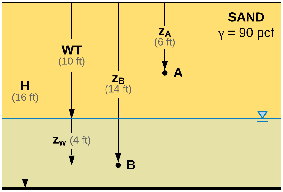
Figure 2 Single layer, stresses above and below water table.

The first takeaway comes with the introduction of the term \(z_w\), the vertical distance below the water table.

Takeaway No 1

\[z_w = z - WT\]

Always calculate \(z_w\) and if negative, set \(z_w=0\). Hence:

\[\begin{split}z_w = \begin{cases} 0 & \textrm{if} \quad z_w < 0 \\ z - WT & \textrm{otherwise} \end{cases}\end{split}\]

Total stress at point A:

\[\sigma_A = \gamma z_A = (90 \textrm{ pcf})(6 \textrm{ ft}) = 540 \textrm{ psf}\]

Pore water pressure at point A:

\[z_w = z_A - WT = 6 - 10 = -4 \textrm{ ft} = 0\]

\[u_A = z_w \, \gamma_w = 0 \textrm{ psf}\]

Effective stress at point A:

\[\sigma'_A = \sigma_A - u_A = 540 - 0 = 540 \textrm{ psf}\]

Total stress at point B:

\[\sigma_B = \gamma z_B = (90 \textrm{ pcf})(14 \textrm{ ft}) = 1260 \textrm{ psf}\]

Pore water pressure at point B:

\[z_w = z_B - WT = 14 - 10 = 4 \textrm{ ft}\]

\[u_A = z_w \, \gamma_w = (62.4 \textrm{ pcf})(4 \textrm{ ft}) = 249.6 \textrm{ psf}\]

Effective stress at point B:

\[\sigma'_B = \sigma_B - u_B = 1260 - 249.6 = 1010.4 \textrm{ psf}\]

The same example can be implemented in edafos as follows.

# Import the `SoilProfile` class
In [1]: from edafos.soil import SoilProfile

# Create a SoilProfile object with initial parameters
In [2]: caseA = SoilProfile(unit_system='English', water_table=10)

# Add layer properties
In [3]: caseA.add_layer(soil_type='cohesionless', height=16, tuw=90)
Out[3]: <edafos.soil.profile.SoilProfile at 0x10f5fe390>

# Stresses at point A
In [4]: total, pore, effective = caseA.calculate_stress(6, kind='all')

In [5]: print("Total Stress: {:0.3f}\nPore Water Pressure: {:0.3f}\n"
   ...:       "Effective Stress: {:0.3f}".format(total, pore, effective))
   ...: 
Total Stress: 0.540 kip / foot ** 2
Pore Water Pressure: 0.000 kip / foot ** 2
Effective Stress: 0.540 kip / foot ** 2

# Stresses at point B
In [6]: total, pore, effective = caseA.calculate_stress(14, kind='all')

In [7]: print("Total Stress: {:0.3f}\nPore Water Pressure: {:0.3f}\n"
   ...:       "Effective Stress: {:0.3f}".format(total, pore, effective))
   ...: 
Total Stress: 1.260 kip / foot ** 2
Pore Water Pressure: 0.250 kip / foot ** 2
Effective Stress: 1.010 kip / foot ** 2

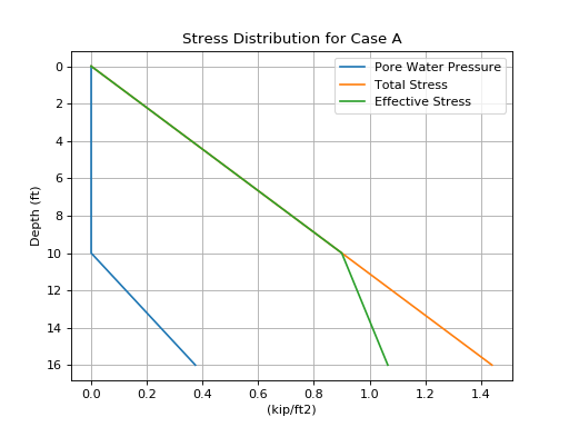
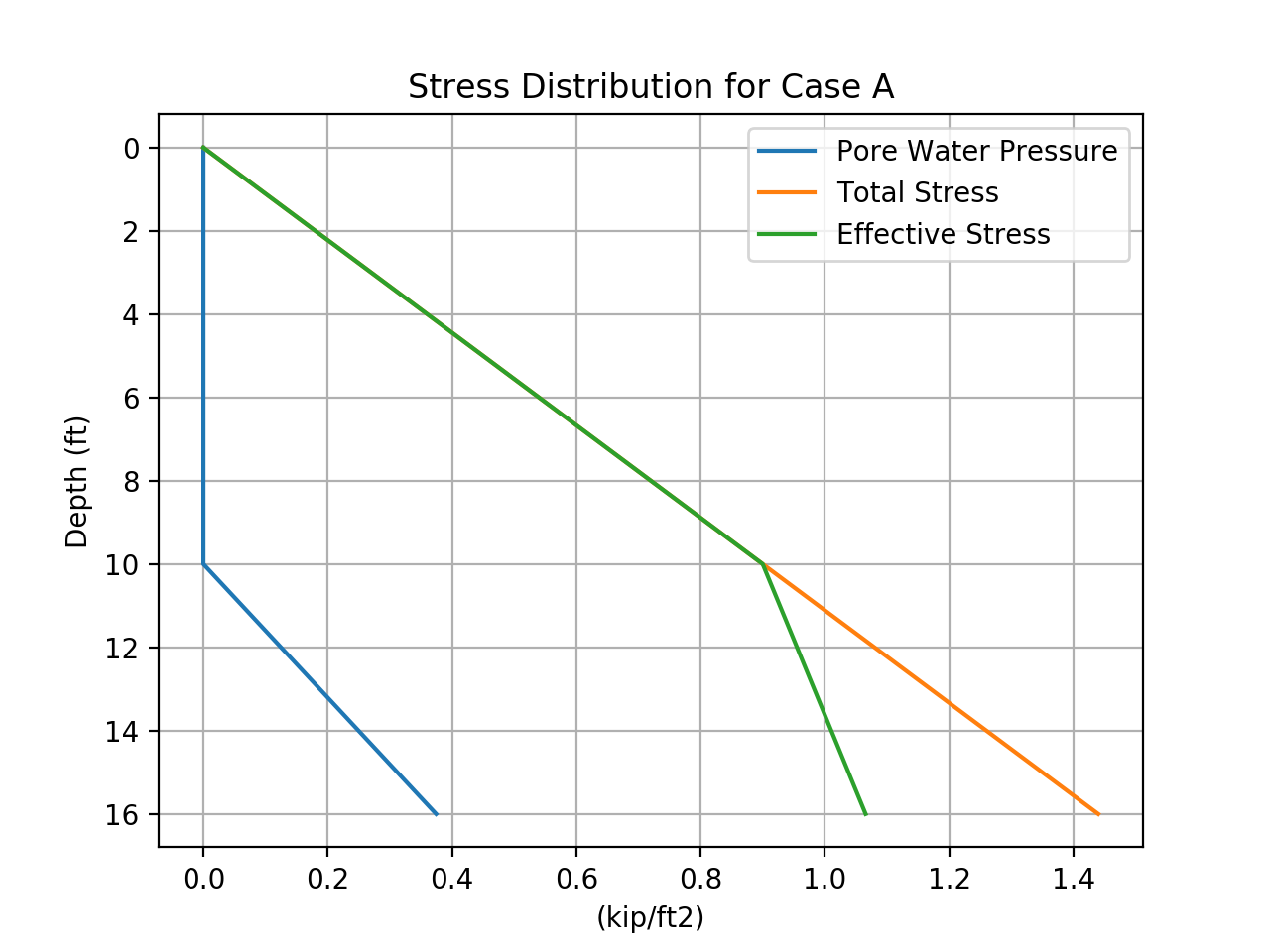
You can also create a stress distribution plot:

(Source code, png, hires.png, pdf)

---

Case B - two layers, stresses above and below water table

Consider the soil profile in Figure 3. A 5-ft sand layer with total unit weight of 90 lbf/ft³, an 11-ft clay layer with total unit weight of 110 lbf/ft³ and the water table at a depth of 10-ft. Point A is at depth, \(z\), of 6-ft and point B is at a depth, \(z\), of 14-ft below ground level.

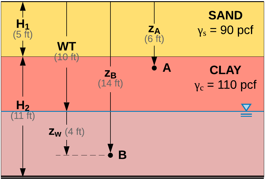
Figure 3 Two layers, stresses above and below water table.

Takeaway No 2

Total stress in terms of \(z\):

\[\begin{split}\sigma(z) = \begin{cases} z \, \gamma_1 & \textrm{if} \quad z < H_1 \\ \sum\limits_{i=1}^n {H_i \, \gamma_i} & \textrm{if} \quad z = \sum\limits_{i=1}^n {H_i} \\ \sum\limits_{i=1}^{n-1} {H_i \, \gamma_i} + \Big(z-\sum\limits_{i=1}^{n-1} {H_i}\Big) \, \gamma_n & \textrm{if} \quad \sum\limits_{i=1}^{n-1} {H_i} < z < \sum\limits_{i=1}^n {H_i} \end{cases}\end{split}\]

Total stress at point A:

\[\sigma_A = H_1 \, \gamma_1 + (z_A-H_1) \, \gamma_2 = (5 \textrm{ ft})(90 \textrm{ pcf}) + (6-5 \textrm{ ft})(110 \textrm{ pcf}) = 560 \textrm{ psf}\]

Pore water pressure at point A:

\[z_w = z_A - WT = 6 - 10 = -4 \textrm{ ft} = 0\]

\[u_A = z_w \, \gamma_w = 0 \textrm{ psf}\]

Effective stress at point A:

\[\sigma'_A = \sigma_A - u_A = 560 - 0 = 560 \textrm{ psf}\]

Total stress at point B:

\[\sigma_B = H_1 \, \gamma_1 + (z_B-H_1) \, \gamma_2 = (5 \textrm{ ft})(90 \textrm{ pcf}) + (14-5 \textrm{ ft})(110 \textrm{ pcf}) = 1440 \textrm{ psf}\]

Pore water pressure at point B:

\[z_w = z_B - WT = 14 - 10 = 4 \textrm{ ft}\]

\[u_A = z_w \, \gamma_w = (62.4 \textrm{ pcf})(4 \textrm{ ft}) = 249.6 \textrm{ psf}\]

Effective stress at point B:

\[\sigma'_B = \sigma_B - u_B = 1440 - 249.6 = 1190.4 \textrm{ psf}\]

Case B can be implemented in edafos as follows.

# Import the `SoilProfile` class
In [8]: from edafos.soil import SoilProfile

# Create a SoilProfile object with initial parameters
In [9]: caseB = SoilProfile(unit_system='English', water_table=10)

# Add layer properties
In [10]: caseB.add_layer(soil_type='cohesionless', height=5, tuw=90)
Out[10]: <edafos.soil.profile.SoilProfile at 0x10fda0b00>

In [11]: caseB.add_layer(soil_type='cohesive', height=11, tuw=110)
Out[11]: <edafos.soil.profile.SoilProfile at 0x10fda0b00>

# Stresses at point A
In [12]: total, pore, effective = caseB.calculate_stress(6, kind='all')

In [13]: print("Total Stress: {:0.3f}\nPore Water Pressure: {:0.3f}\n"
   ....:       "Effective Stress: {:0.3f}".format(total, pore, effective))
   ....: 
Total Stress: 0.560 kip / foot ** 2
Pore Water Pressure: 0.000 kip / foot ** 2
Effective Stress: 0.560 kip / foot ** 2

# Stresses at point B
In [14]: total, pore, effective = caseB.calculate_stress(14, kind='all')

In [15]: print("Total Stress: {:0.3f}\nPore Water Pressure: {:0.3f}\n"
   ....:       "Effective Stress: {:0.3f}".format(total, pore, effective))
   ....: 
Total Stress: 1.440 kip / foot ** 2
Pore Water Pressure: 0.250 kip / foot ** 2
Effective Stress: 1.190 kip / foot ** 2

You can also create a stress distribution plot:

(Source code, png, hires.png, pdf)

---

Case C - two layers, under water

Consider the soil profile in Figure 4. A 4.5-ft sand layer with total unit weight of 90 lbf/ft³ and a 4.5-ft clay layer with total unit weight of 110 lbf/ft³ are under 7-ft of water. Point A is 3-ft above soil grade and point B is at a depth, \(z\), of 7-ft below soil grade.

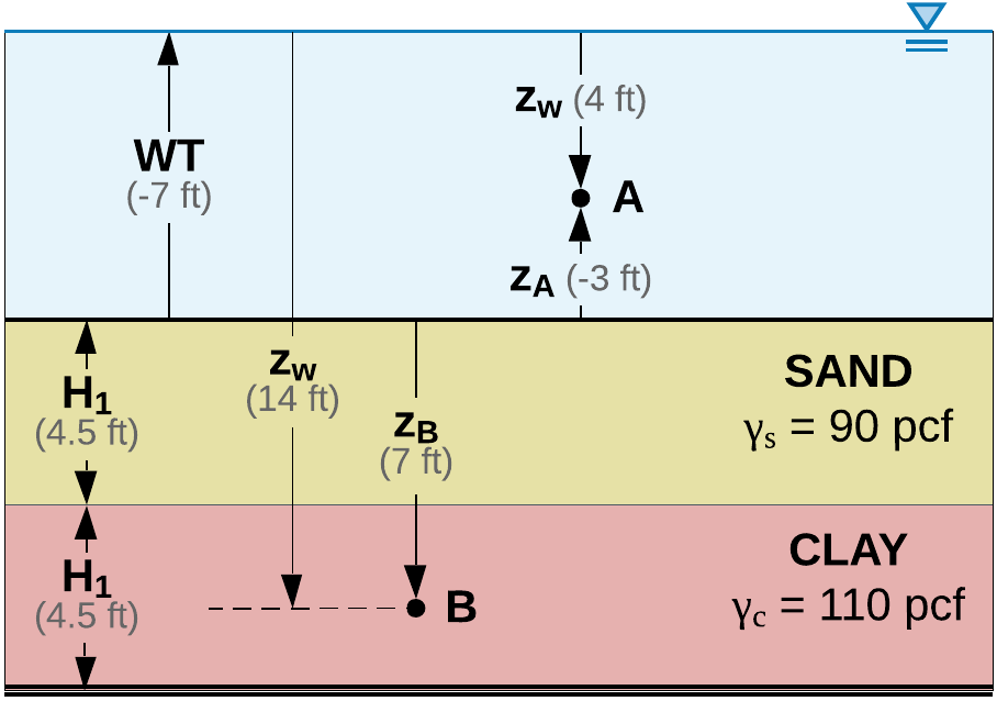
Figure 4 Two layers, under water.

Total stress at point A:

\[z_w = z_A - WT = -3 - (-7) = 4 \textrm{ ft}\]

\[\sigma_A = z_w \, \gamma_w = (4 \textrm{ ft})(62.4 \textrm{ pcf}) = 249.6 \textrm{ psf}\]

Pore water pressure at point A:

\[u_A = z_w \, \gamma_w = (4 \textrm{ ft})(62.4 \textrm{ pcf}) = 249.6 \textrm{ psf}\]

Effective stress at point A:

\[\sigma'_A = \sigma_A - u_A = 249.6 - 249.6 = 0 \textrm{ psf}\]

Takeaway No 3

If \(z<0\) and \(WT<0\), then:

\[\sigma = u = z_w \, \gamma_w\]

Total stress at point B:

\[\sigma_B = | WT | \, \gamma_w + H_1 \, \gamma_1 + (z_B-H_1) \, \gamma_2 = (7 \textrm{ ft})(62.4 \textrm{ pcf}) + (4.5 \textrm{ ft})(90 \textrm{ pcf}) + (7-4.5 \textrm{ ft})(110 \textrm{ pcf}) = 1116.8 \textrm{ psf}\]

Pore water pressure at point B:

\[z_w = z_B - WT = 7 - (-7) = 14 \textrm{ ft}\]

\[u_B = z_w \, \gamma_w = (14 \textrm{ ft})(62.4 \textrm{ pcf}) = 873.6 \textrm{ psf}\]

Effective stress at point B:

\[\sigma'_B = \sigma_B - u_B = 1116.8 - 873.6 = 243.2 \textrm{ psf}\]

Takeaway No 4

If \(z>0\) and \(WT<0\), adjust the total stress equation to include above grade stresses due to water pressure.

Case C can be implemented in edafos as follows.

# Import the `SoilProfile` class
In [16]: from edafos.soil import SoilProfile

# Create a SoilProfile object with initial parameters
In [17]: caseC = SoilProfile(unit_system='English', water_table=-7)

# Add layer properties
In [18]: caseC.add_layer(soil_type='cohesionless', height=4.5, tuw=90)
Out[18]: <edafos.soil.profile.SoilProfile at 0x11071e470>

In [19]: caseC.add_layer(soil_type='cohesive', height=4.5, tuw=110)
Out[19]: <edafos.soil.profile.SoilProfile at 0x11071e470>

# Stresses at point A
In [20]: total, pore, effective = caseC.calculate_stress(-3, kind='all')

In [21]: print("Total Stress: {:0.3f}\nPore Water Pressure: {:0.3f}\n"
   ....:       "Effective Stress: {:0.3f}".format(total, pore, effective))
   ....: 
Total Stress: 0.250 kip / foot ** 2
Pore Water Pressure: 0.250 kip / foot ** 2
Effective Stress: 0.000 kip / foot ** 2

# Stresses at point B
In [22]: total, pore, effective = caseC.calculate_stress(7, kind='all')

In [23]: print("Total Stress: {:0.3f}\nPore Water Pressure: {:0.3f}\n"
   ....:       "Effective Stress: {:0.3f}".format(total, pore, effective))
   ....: 
Total Stress: 1.117 kip / foot ** 2
Pore Water Pressure: 0.874 kip / foot ** 2
Effective Stress: 0.243 kip / foot ** 2

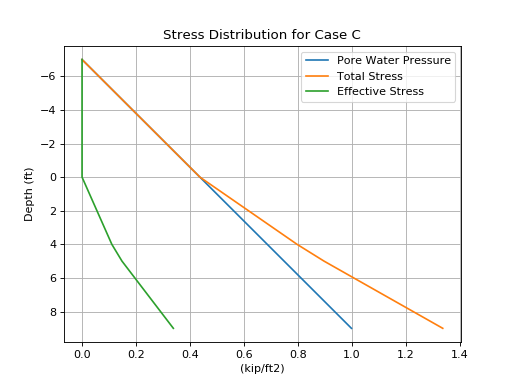
You can also create a stress distribution plot:

(Source code, png, hires.png, pdf)